
One failure can prove that a model made a mistake. It cannot, by itself, prove that the model fails more often than it used to.
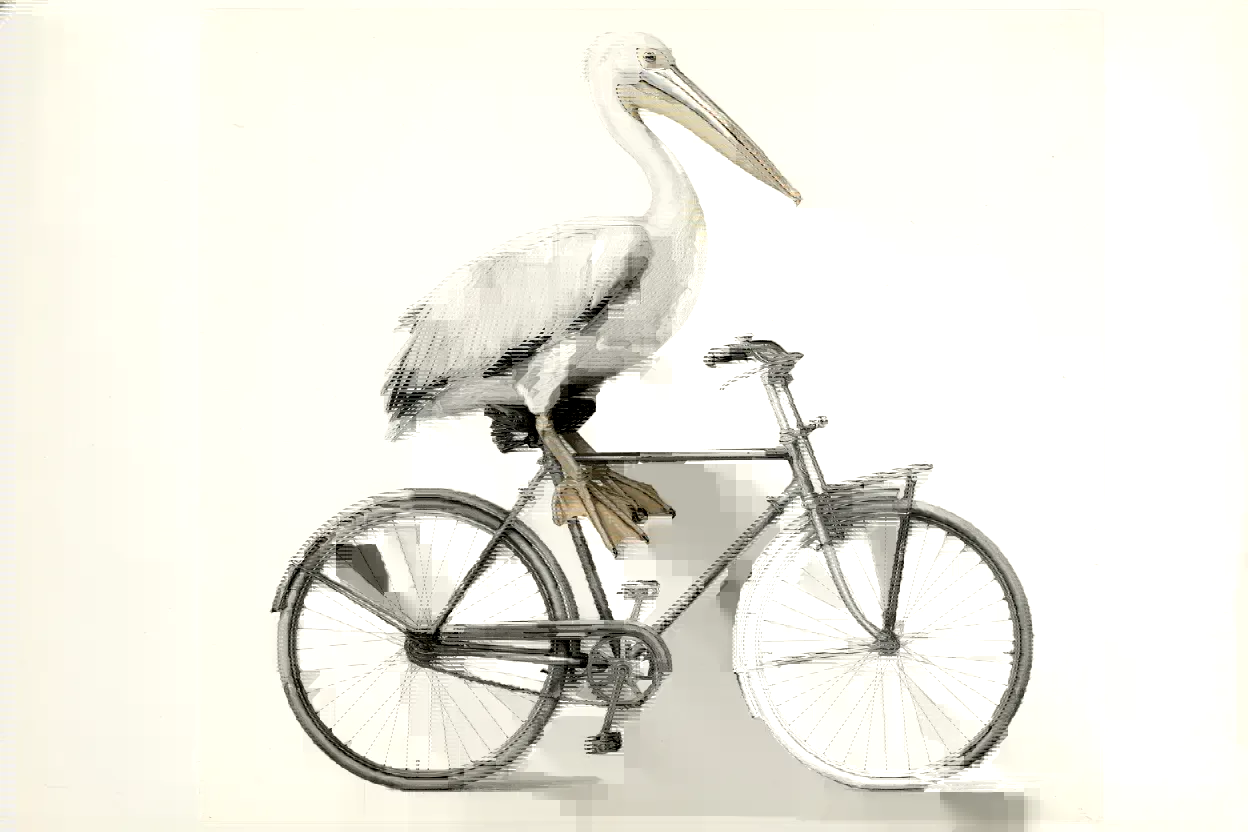
“Did this model get dumber again?” A pelican with one foot hanging off the pedal, a bicycle whose frame is twisted into a knot, set beside a screenshot that looked quite good last week: that is enough to raise the question.
That suspicion should not be waved away with “models are random.” Someone paid for a task the service used to finish, and now it does not. That is worth asking about. Two screenshots, though, are not enough to show that the model was swapped, that the thinking budget was cut, or that a particular service was watered down.
A while ago I ran the pelican test dozens of times. What makes the task useful is that many of its mistakes are drawn where you can see them. Code that runs does not mean the bicycle is structurally right. A bird and a bicycle that are both present do not mean the foot is actually on the pedal. Those spatial relationships are easier to catch by eye than a fluent answer that may still hide a logical hole. The more runs I kept, the clearer another point became: we often judge an entire service by a single piece of work.
This article is not here to excuse any model, and it does not teach anyone to spot a “fake model” from a few surface traits. The question I care about is narrower. When we suspect that a model has gotten worse, how do we turn that feeling into evidence someone else can recheck?
Note: services A and B below, and every test number attached to them, are teaching examples. They do not refer to any real service, and they are not a Folkbench measurement or ranking.
1. First separate the question: what do you mean by “dumber”?
“Got dumber” is a convenient phrase, and it folds several different questions into one. The most direct layer is: this particular answer is wrong. The pelican grew an extra leg, the foot missed the pedal, or the wheels came apart from the frame. Each of those is a concrete failure you can check. One sample is enough to prove that “this kind of error happened,” and enough to defeat a promise that “it would never make this kind of error.” The second layer is: under the same conditions, or conditions close enough, this service fails more often.
That is no longer a question of whether the error exists. It is a question of how often it appears. The part of “the experience got worse” that is most worth measuring is the shift from “it usually worked” to “it usually does not.” The third layer is: the change was caused by a change in the model itself, or in the server-side configuration. That is already a claim about cause. The same bad result can come from different explanations: different request parameters, different context, a truncated output, or a real change in the underlying model and inference settings. Seeing the result alone usually cannot single one of those explanations out.
So “this one was wrong,” “this service is less reliable,” and “this service quietly swapped the model” do not call for evidence of the same strength. Noticing that difference does not raise the bar for a user’s complaint. It does the opposite. Naming the question clearly keeps a provider from explaining every failure as “randomness,” and keeps an evaluator from explaining every difference as “they swapped the model.”
2. Are you looking at one piece of work, or at a distribution of outputs?
Under a generation setting that samples at random, the same input can produce different outputs. Even when you use some control meant to improve reproducibility, “as consistent as we can make it” should not be read as “identical every time.” An older OpenAI technical note said this explicitly: with the same seed, the same parameters, and the same backend fingerprint, the output is still not guaranteed to be identical. That is a boundary on reproducibility. It does not mean every model today accepts the same parameters.1
For the pelican test, what we usually want to know is not “can it occasionally draw one good picture?” It is “under the conditions I specified, if I hand it the task once more, how likely is a qualified result?” A simplified example shows the problem with a single screenshot. Suppose a service’s true single-try qualification rate is 80%, each generation is independent, and its state does not change during the test. The probability of at least one failure in 20 consecutive tries is: 1 − 0.8²⁰ ≈ 98.85% A service that usually does the job well will almost certainly leave behind a failure you can screenshot, somewhere in those 20 tries.
Turn it around. Suppose another service’s true single-try qualification rate is only 40%. Under the same assumptions of independence and stability, the probability of at least one qualified result in 20 tries is: 1 − 0.6²⁰ ≈ 99.996% It, too, will almost certainly produce one piece of work you can hold up. These two calculations do not say that every real call is independent, and they do not say that real qualification rates are exactly these numbers. They point at a choice: showing only the best try makes reliability easy to overstate, and showing only the worst try makes a decline easy to exaggerate.
The same service can therefore appear in a post that treats one image as proof it is at full strength, and in another that treats one image as proof it got dumber. Both screenshots can be real. The inference does not have to be. There is another distinction that is easy to skip. Succeeding on the first generation, and generating ten times and then picking the success, are not the same capability. The second includes extra calls, waiting, and the cost of selection. If you compare two workflows, give both the same attempt budget. Do not compare A’s first try with B’s curated favorite.
3. Does 20 runs automatically make a difference statistically meaningful?
No. Twenty runs can be a reasonable experimental budget. They are not a statistical permit. Take the same concrete example. Channel A is run 20 times and qualifies 16 times. Channel B is run 20 times and qualifies 8 times. Both use one fixed task and the same scoring rule, and every sample is kept.
| Channel | Qualified / total | Sample rate | 95% Wilson interval for the rate |
|---|---|---|---|
| A | 16 / 20 | 80% | 58.4%–91.9% |
| B | 8 / 20 | 40% | 21.9%–61.3% |
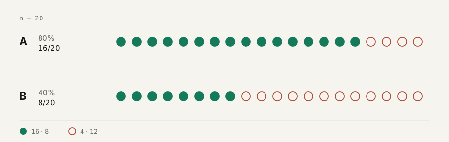
The intervals are two-sided 95% Wilson intervals for a binomial proportion. They express uncertainty in the estimated qualification rate. They are not a score range for picture quality.2 The difference in the sample is 40 percentage points. With only 20 tries on each side, the estimate is still coarse. 80% and 40% should not be treated as a true ability that has been measured exactly and will never move.
If we further assume that calls are independent, that each channel’s qualification probability is stable inside the window, and that this comparison was chosen in advance, a two-sided Fisher’s exact test on the qualified / not-qualified counts gives p ≈ 0.0225. At a 5% significance level chosen beforehand, this example supports “the qualification rates differ under these conditions.”3 That number is not “a 97.75% chance that B was watered down,” and it is not “a 97.75% chance that A is forever better.” A p-value is the probability of data this extreme, or more extreme, under a no-difference hypothesis and the conditions of the test. It is not the probability of a hidden cause.3
Do not replace a test of the difference with a glance at whether the two intervals overlap. Each interval estimates one rate. The test is about the difference between them. Three boundaries matter more than memorizing one test. Look at the size of the gap and the sample size together. 16 against 8 should not support a conclusion of the same strength as 16 against 15. How many samples you need depends on how small a gap you hope to detect, and on how much risk of a wrong call you will accept. There is no “run it at least this many times” that fits every task.
Failing to find a significant difference does not prove the two are the same. The data may simply be too few, or too unstable, to support a conclusion yet. To show that a difference is small enough to ignore, define “small enough” in advance. An insignificant result is not a proof of equivalence. A statistical difference is not, by itself, a reason to switch services. A user still has to weigh the cost of a failure, the price of a call, the latency, and the cost of doing the work again. A difference can be real and still too small to change the choice. The job of the statistics here is not to produce a p-value that looks professional. It is to stop us from claiming more than the evidence can carry.
4. A baseline is an experimental contract, not the sentence “the prompt was the same”
Many comparisons fail before the sample size becomes the issue. The samples were not comparable from the start. Both sides are asked to “draw a pelican riding a bicycle.” One call is an API request in a fresh session. The other is a chat window dozens of turns deep, with tools turned on. One side may write a long output. The other hits a length limit halfway through. Repeating that a hundred times still does not let you attribute the result to a difference in model ability.
Research on the OLMES evaluation standard points out that evaluation choices such as prompt format, in-context examples, and task wording change the performance you measure. A reproducible comparison has to record those settings. The tasks in that work are not the pelican SVG, but the warning about experimental configuration is worth taking.4 I would treat the baseline as a contract for “what this round is actually measuring.”
The thing being compared should be specific: the service, the group or route, and the model version you can actually obtain. If all you have is a model alias that can change over time, record the alias. If you do not know the underlying snapshot, write unknown. Do not treat the model string returned by the interface as independent verification of the underlying identity. Save the input as completely as you can. That means more than the final prompt. It includes the system prompt, history, attachments, and tool settings you can control and observe. Matching the visible conditions does not prove that the invisible conditions matched.
For the generation settings, record the thinking effort, the output limit, and the sampling parameters the interface actually supports. Write “unsupported” for a field the interface does not offer, and “unknown” for a field you cannot confirm took effect. Do not quietly treat those as matched. A setting named “high” should not be assumed to mean the same compute budget on two different models.
The evaluation environment includes how you render and how you score. Check the same SVG in the same viewport and renderer. For an animation task, use the agreed observation window. Do not watch the full motion on one side and pick a single frame on the other. If the task did not ask for animation, do not deduct points because the output is a still image. Finally, write the retry rule before the test starts. Whether a first failure may be retried, how many times, and whether feedback is allowed, are part of the test conditions. They are not something to improvise once the results are in.
Fixing these things is not an attempt to build a “laboratory model” that has left the real world. You can absolutely compare the default experience of two chat products. The conclusion should then be “these two products differ in what they deliver under default settings,” not “I have isolated which underlying model weights are better.” A condition you cannot control can stay unknown. An unknown condition cannot be written down as controlled.
5. How you arrange the test often matters more than simply running it more times
Do not tie the channel to the time of day
Running all of A in the morning, then all of B late at night, mixes “a difference between channels” with “a difference across time.” Even if you do see a gap, it is hard to say how much of it depends on that window. For a light side-by-side comparison, I would interleave A and B inside a window chosen in advance, and randomize the order. Keep the concurrency as similar as you can. Do not let one side generate one at a time while the other absorbs a burst.
You can go one step further and split the window into small batches, with both A and B in every batch. Besides the overall result, you can then see whether the difference is concentrated in a single batch. A random order helps reduce confounding by time. It does not automatically remove correlation from a shared backend, a short outage, or anything similar.
A longitudinal question, “is it worse than last week?”, is different. Time is the variable you are studying, so you cannot pin both sides to the same moment. Keep the same core task, configuration, and scoring rule as far as you can, and rerun a reference service inside every observation window. Do not forever compare today’s results with last week’s single best image. When you read a longitudinal result, keep both the absolute qualification rate and the relative gap. If the service under test and the reference both drop, the gap between them may stay the same. That does not mean the user’s experience did not get worse. A reference is not a truth that is forever correct and forever stable.
Do not decide when to stop while you are looking at the results
“Run five times. If A wins, post it. If A does not win, keep going until the difference is significant.” That looks like adding samples. It changes the statistical rule. Peeking at a fixed-sample test over and over, and stopping because of what you see, breaks the false-positive control that test was built for. A test that needs to watch the data continuously should use a method designed for sequential analysis.5 Most people do not need to start with sequential statistics. The easiest practice is to write down, before the round, how many runs you will make, which primary metric you will use, and which primary comparisons you will make. Then keep every result.
Trying a few calls first, to confirm that the interface and the scoring process work, is fine. Those are pilot runs. Once you finish changing the procedure, start the formal test on its own. Do not mix the results from tuning the task with the formal results. The same point covers two other habits. Trying dozens of tasks and publishing only the one that looks best, or seeing that the total score is behind and then declaring victory on a subscale, is not the comparison you agreed to in advance.
Do not treat a hundred repeats of one task as a hundred tasks
Repeated generation tells you how reliable the service is on this task. It does not automatically widen the claim. A pelican that comes out steadily does not, by itself, mean that code debugging, long-form analysis, and complex instruction following are equally reliable. When you infer about a class of tasks, variation between tasks and variation across repeats of one task are two different kinds of uncertainty. Evaluation research distinguishes repeated sampling, comparisons at the level of the task, and the handling of clustered, dependent samples.6
So I would first use one probe to watch repeatability, then add a small set of fixed tasks tied to the actual use. Both sides answer the same set. Compute the result on each task, and the difference on each task, before you aggregate. Do not throw out only a total score. If you run a formal analysis on several tasks, keep the pairing of the same task and the same batch. You cannot treat “10 tasks, 10 times each” as “100 independent tasks” and reuse the single-task calculation from earlier.
There is a smaller trap. A fixed seed is useful when you are chasing a reproduction problem. Copying an almost unchanged output from the same seed twenty times is not twenty independent observations of the random output distribution. When you are measuring stability, agree on the sampling strategy beforehand. An interface that supports seeds can use several seeds generated in advance. An interface that does not should have that limit recorded. How a task set should be updated over the long run is a separate question. At least inside this one comparison, do not change the tasks and then connect the old and new scores into a “the model is improving” curve.
6. Timeouts, truncation, and a wrong drawing do not belong in one pile
A common statistical distortion is to score only the pieces of work that came back successfully, and to delete timeouts and errors. The score you get answers “once a complete output is in hand, how often is it qualified?” It does not answer the question a user cares about more: “if I send one request, do I get a qualified result?” Suppose 20 requests were arranged in advance, and 4 of them timed out. The other 16 returned a complete piece of work, and 8 of those were qualified. The qualification rate among complete outputs is 50%. The rate of a qualified first delivery, counted over all 20 requests, is 40%. Publishing only the first number leaves out the four times the user received nothing.
I would keep three kinds of result at once: a technical failure to deliver, a complete return that fails the task, and a complete return that passes the task. Timeouts, interface errors, interrupted streams, and hitting the length limit should each keep their own reason. Recording them separately does not excuse a service failure. For someone choosing a service, a timeout and a wrong drawing both cost time. When you are tracing a cause, though, they should not all be described as “the model’s intelligence declined.” A fault in the local network or in the test script should be listed on its own. Whether to exclude it needs a rule written beforehand. You cannot delete a sample after you see which side lost.
I would rather make the share of first requests that return a qualified result the primary metric, and keep the content-qualification rate among complete outputs, the technical failure rate, the latency, and the cost alongside it as explanations. The content-qualification rate on complete outputs is not an unbiased “pure ability” score either. If complex requests are more likely to time out, the work that remains may have been easier to begin with. That rate can help locate a problem. It cannot replace the result counted over every request.
“Can it succeed after one repair?” can be a separate test, with the same chance to repair on both sides. Do not coach one side through five rounds of correction and condemn the other at the first mistake.
7. A minimal comparison an ordinary person can actually run
You do not need to build an evaluation platform before you test one pelican. Here is a starting plan. It is for checking an obvious difference on one fixed probe. It is not a sample-size design that guarantees you will detect a small decline.
| Item | Agreement for this round |
|---|---|
| Question | On this fixed task, do services A and B differ in the share of first deliveries that are qualified? |
| Input and settings | Save the full visible request. Match the parameters you can control. Record differences you cannot confirm. |
| Sample | Arrange 20 formal requests on each side in advance. Keep pilot runs out of the formal sample. |
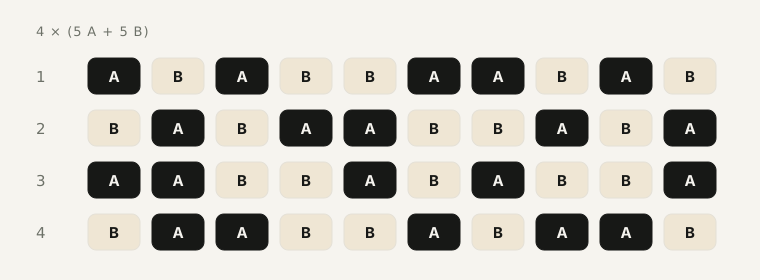
| Time and order | Split a predeclared window into 4 batches, with 5 calls each for A and B. Interleave them at random inside the batch, under the same concurrency rule. |
| Retries | The formal first-answer test adds no retry. Open a separate experiment if you want to measure repair. |
| Scoring | Fix the qualification rule before the first run. After rendering, hide the channel name, shuffle the order, and then score. |
| Output | Save every raw result, the status of each call, the reason for each score, and both the per-batch and overall statistics. |
A plain qualification rule is a good place to start for the pelican task. Does the file render in the agreed environment? Are the subject and the bicycle complete enough to recognize? Is a key structure obviously wrong? Do the contacts the task requires, such as foot and pedal, actually hold? You can note beauty separately. Careful color cannot cancel a structural error.
If someone is unsure about a borderline sample, mark it as disputed and follow the review rule you set in advance. Do not decide whether it passes after you have seen the channel name. A small test can be scored by hand, blind. Once the scale grows, automated scoring and judge calibration are the next question. They do not all have to be solved in round one. Recording is much easier if you separate the configuration that belongs to the round from the log that has one row per call. The round configuration keeps the raw request template, the parameters, the task version, the scoring-rule version, the time window, and the timeout and retry agreement. Each call should record at least these fields:
run_id,block_id,service,service_group,requested_model,returned_model,started_at,request_hash,status,finish_reason,latency_ms,qualified,failure_reason,artifact_pathWrite times with a time zone. Relate the raw response, the extracted SVG, and the rendered image through artifact_path. Token counts, backend fingerprints, and anything else the interface exposes can be stored alongside. If it was not provided, record it as empty or unknown. request_hash is a check that the request stayed the same. It does not replace the raw request. When you save or share the log, remove API keys, and redact private context or other sensitive content. What a public check needs is the experimental conditions, not the account credentials handed over with them.
When you summarize, look first at the overall gap and at the result of each batch. The binomial interval and Fisher’s exact test from earlier apply when their assumptions, including independence and stability, roughly hold. If the result is clearly affected by the batch, or if you later expand to repeated tests on several tasks, analyze the matched design. Do not reuse the single-task formula mechanically. If a first difference is worth chasing, retest it in a new predeclared window, and add tasks related to the use you actually have. The first round is a lead on an anomaly. A separate new round is what helps you judge whether it is still there.
8. After you find a difference, how should the conclusion be written?
Using the same teaching numbers, a restrained and still useful conclusion can read like this:
Under this round’s fixed task, matched visible settings, and predeclared time window, A and B were each tested 20 times. Qualified first deliveries were 16 and 8. The sample qualification rates differ by 40 percentage points. Under assumptions that include independent sampling, a two-sided Fisher’s exact test gives a p-value of about 0.0225, which supports a difference under this round’s conditions. The result still needs to be checked in other windows and on related tasks. It cannot, on its own, identify the specific cause of a change in the underlying model or in the server configuration.
It is less exciting than “proof it is at full strength.” It does hand the next person the conditions they need in order to recheck it. If later tests, across time and across related tasks, keep pointing the same way, we have a stronger reason to say that this service is less reliable than the reference for these uses, or that it really has fallen behind its own historical baseline. Jumping from “delivery got worse” to “they quietly swapped in a smaller model” is still an extra step. Confirming a specific mechanism needs independent evidence that can tell the explanations apart, such as a route or configuration record you can verify. Output style is not enough to guess the model.
That also does not mean a user has to wait until the cause is known before they are allowed to switch. Choosing a service depends on whether it meets your requirements. Accusing a specific cause depends on evidence about that cause. The two can stay separate.
9. What is actually worth saving is the cost of proving the question clearly
The tiring part of a manual test is usually not pressing run. It is the repeated work afterward. Where is the file? Did the parameters change? Which generation is this image? Was it a retry? Can the screenshot still be matched to the raw response? Without those records, a conviction that “it really got dumber” can, a week later, be nothing but a few screenshots nobody can recheck.
If you only want a first look at how different services behave, not everyone has to organize that from zero. You can start at Folkbench and look at the public rankings and the way into the reports, and see whether the model, service group, and metric you care about already have a result. The public pages emphasize comparing services under the same model, and the rankings also say that the numbers in one row’s group do not stand for every group at that station.7
A published board should reduce the cost of collecting and organizing. It should not be a reason to stop checking the conditions. Folkbench included, any ranking is worth asking further: when was it measured, what was measured, how large was the sample, were the failures kept, and what range does the conclusion cover? Information that is not public is still unknown. Back to the opening question. How much of “the model got dumber” is real, and how much is the illusion of a single draw?
Before there is a shared definition, a complete sample, and comparable conditions, publishing one overall percentage only creates a new piece of folklore. What we can do better is take each concrete suspicion and turn it, step by step, into a judgment that can be checked. When you see a failure, keep the raw result. When you suspect a decline, start a comparison. When you find a difference, then trace the cause. Do not try to finish all of those steps inside a single screenshot. A screenshot can ask a good question. Answering it still takes a decent experiment.
Notes and sources
- OpenAI, How to make your completions outputs consistent with the new seed parameter, an archived Cookbook example. The note describes a fixed seed as a best effort toward determinism, not a guarantee. This article cites only that boundary on reproducibility. It does not treat the older model names or the parameter support in that page as a current product description. Source↩
- NIST/SEMATECH, e-Handbook of Statistical Methods, section 7.2.4.1, Confidence intervals, Wilson score interval for a proportion. This article uses two-sided 95% Wilson intervals for 16/20 and 8/20. The author computed them from the formula and rounded to one decimal place in percent. The confidence level describes the long-run coverage of the interval method. The Wilson method is an approximation. Source↩
- SciPy documentation,
scipy.stats.fisher_exact. This article uses the contingency table[[16, 4], [8, 12]]withalternative="two-sided"and getsp = 0.0224774273717544. That is a calculation on the example data, not a measured result from a paper or a platform report. The example compares independent binomial outcomes. Paired data, clustering across tasks, time dependence, or multiple comparisons need an analysis that matches the design. Source↩ - Yuling Gu et al., OLMES: A Standard for Language Model Evaluations, Findings of NAACL 2025. The paper discusses evaluation details such as prompt format, the choice of in-context examples, and task wording, and what a reproducible comparison requires. Source↩
- Ramesh Johari, Leo Pekelis, and David J. Walsh, Always Valid Inference: Bringing Sequential Analysis to A/B Testing, arXiv:1512.04922, 2019 revision. The paper discusses the problem of watching results continuously and letting that decide the sample size, and the sequential inference methods that address it. Source↩
- Evan Miller, Adding Error Bars to Evals: A Statistical Approach to Language Model Evaluations, 2024. On uncertainty at the task level, repeated sampling, paired comparisons, and clustered samples, see sections 2, 3, and 4. On sample-size planning, see section 5. Source↩
- Folkbench’s public home and rankings pages, checked on 5 October 2026. This article uses those public pages only to describe the entry point, the scope of comparison, and the group-level notice. It does not independently endorse any specific ranking number, and it does not say that Folkbench already implements every experimental procedure proposed here. Home; Rankings↩